
This is the second post in a short series, presenting my work for CERN during this year’s google summer of code. Having just finished the first CUDA implementation of the convolutional network library, I will iterate over the major considerations I had to take into account when testing that implementation. It should be noted that asserting correctness in as many scenarios as possible is crucial for any piece of software that is even remotely complex. Below we will see what this requirement entails in a machine learning context.
One of the tasks that I had to address at a preliminary stage, is to split to library into a discrete set of features. What I have found to be extremely important when dividing a complex problem, is to ensure that each piece is inherently self-contained. This enables one to implement each feature with minimal concerns regarding external parts, as well as test it in isolation. Let’s contrast this approach with the following scary scenario:
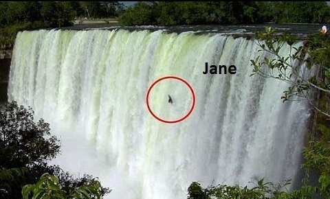
Horror movie plot: Jane starts working on a convolutional neural network library. She follows a waterfall model where each part is developed one after the other. At the end she arrives at a library that compiles without an error. She designs a simple network architecture, and tests it on a given dataset. She soon finds out that the loss is sadly not decreasing as the training epochs progress. Does this mean that:
I had to tackle all of those errors (yes even the 4th one!) while developing each piece in isolation. Detecting each of them while testing the network as a whole, is arguably harder than developing the library in the first place!
 Jane following the waterfall model
In order to protect my sanity, I decided to divide the library into parts, each of which is manageable in isolation. A rather logical division strategy, is to assign a “one-man sprint” per layer type:
Splitting the end product into the aforementioned pieces affects the following facets of the development process (this is the last list in this post I promise):
In our context, unit testing refers to numerically asserting the expected behavior of each function. Fortunately, each layer type only contains two testing-worthy functions: Forward and backward propagation. Let’s make that clear with a concrete example: How would one test the forward-propagation of a max-pooling layer? We start by defining the expected behavior.
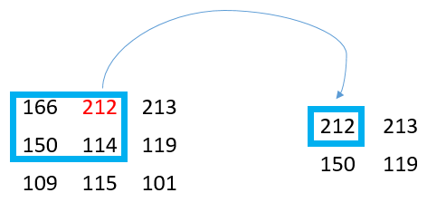
The max pooling layer slides a kernel over its input. At each stage it selects the neuron with the maximum value within the current receptive field and assigns it to the output.
If the above definition is not entirely clear, the reader is encouraged to check the notes from the brilliant course delivered by Stanford. We can therefore design a simple test. Let’s set the input to a single 3 by 3 feature map. The stride will be equal to 1, and the padding to 0.
 Input: 3x3, stride = 1, padding = 0. Therefore Output: 2x2
We can then test directly: assert expected == pooling.forwardPropagation(input)
Of course our library ought to support every valid configuration, therefore these should also be covered by our testing suite. In a realistic scenario we would expect the input to span multiple feature maps, the stride to be higher than 1 and maybe not even symmetrical between the vertical and horizontal dimensions. The padding could be adapted to control the output size. The fact that the first simple test passed does not guarantee correctness in the general case! The same process is then followed for both the forward and back propagation of all supported layer types.
We have now written all the required unit tests: each individual piece of work is working as expected. We can now sleep lightly. Wrong! If there is one thing I remember after 6 years in electrical engineering, it is the fact that a system is more than the sum of its counterparts. Besides the 32 bit OP code for addition on a MIPS micro-controller of course - apparently thats important knowledge for an electrical engineer. Aaanyway… What this means is that asserting correctness of each individual layer type in isolation, does not guarantee that the network as a whole will be able to learn. We need to test how these pieces operate when orchestrated. Are the gradients correctly computed? Is the loss actually minimized?
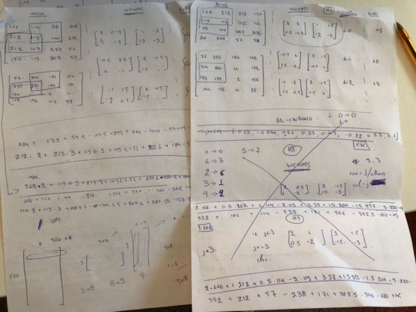
My first thought was to follow the same strategy at the integration stage as well, since it served me perfectly during unit testing. The process would look like this: One would assign arbitrary input and weight values for each layer of a neural network. That network should include at least one layer of each type. The depths must be greater than 1 and the strides asymmetrical to make sure we are checking all cases. One would then propagate the input through the network and compute the output of each layer on paper. Warning bells start ringing for most sane people at this step. The last step would entail performing back-propagation on paper, by computing the activation and weight gradients on paper for each layer. On paper. After trying step 2 (see image below), my honest estimation is that an expert would need to devote about two weeks of her time performing multiplications and convolutions by hand to reach a wrong result because of arithmetic errors.
 Forward propagation on paper, pages 2 of 1
I was actually stubborn enough to perform step 2. It took me three days and I made more than five arithmetic errors on the paper solution. I removed “attention to detail” from my CV header and decided to move on with my life.
I was fortunate enough to observe a brilliant existing implementation written some years ago by Simon Pfreundschuh and adapted to convolutional networks by Vladimir Ilievsky, of a technique called Gradient Checking. The idea is pretty simple, one only needs to remember that all we need back-propagation for, is to compute the gradient of the loss with respect to each individual learnable parameter in the network. The fact that most implementations (including ours) also compute the gradients with respect to each layer’s activation is irrelevant: These are only an intermediate result needed to propagate the error to a previous layer. We are not interested in them directly. Using this simple observation we can then dig into our high school memories and find the definition of that gradient we are so eager to compute:
 Derivative definition
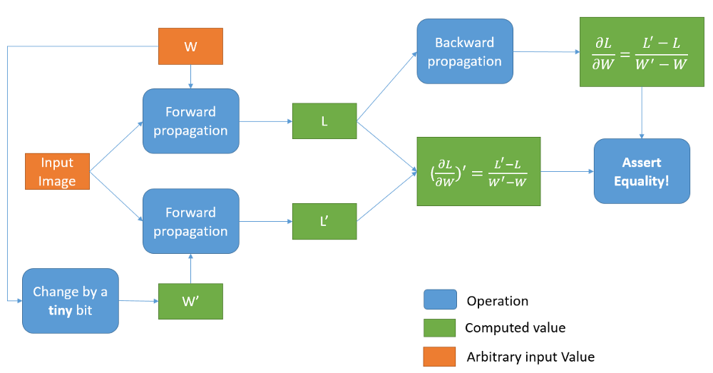
This equation is rather easy to interpret: A weight’s gradient expresses how much the total loss would change, if we were to modify the weight itself by a tiiiny tiny bit. Well why don’t we do exactly that?! Here is a diagram of the proposed process:
 Gradient Checking
We start by arbitrarily setting the orange stuff: an input image and the weights W for every layer. We then perform forward propagation and get the total loss L. We also change the weights by a tiiiiny tiny bit (that’s how I call dW), perform forward propagation using the same image, and get the new loss L’. The ratio of the change in the loss, divided by the change in each weight, is this particular weight’s derivative! All we then have to do, is perform backward propagation using the initial loss L, and get the computed weight gradients. If both those methods of computing the gradients yield the same result, we can be confident that our network works (assuming that forward propagation is correct).
I was delighted to discover that after minor tweaking, my CUDA implementation passed the aforementioned tests. I am now pretty confident on its correctness and feel ready to start tuning for performance. My short term goal is to at least outperform the CPU version (should be easy in theory). I will also try to benchmark the implementation against popular packages such as Tensorflow. It would be great if ROOT could beat some or all of them at least in the context of particle physics experiments, but it is too early to reason about the implementation’s potential.
The library not only outperforms the previous CPU implementation by a factor of 3, but also yields results comparable to industry standards such as Keras. For details, check my final report for GSoC